This is a bonus report following my previous reports on stage 1. This report is about another attempt to get a longer video file decoded in order to get a more realistic use case for testing.
To start off, this time around I was able to successfully convert a mp4 file to a raw .264 file. The method used was to use the file conversion site called Convert.Files where I was able to upload an mp4 file and convert it to a .264 file.
Unfortunately when it came to running the decoder for my test case I came across numerous error messages that made me question the validity of the times outputted. As I was concerned whether any type of decoding operation was actually performed.
Due to these issues I am very likely to stick with my currently submitted used case and testing results.
The results: https://gist.github.com/Megawats777/34c3aaf875af6fa44417c90db0f61e1f
Thank you for reading.
Sunday, March 29, 2020
Tuesday, March 24, 2020
Final Project - Stage 1 Report (Follow Up)
This is a follow up from the previous report on stage 1. The reason for this follow up was that I had a discussion with my professor on what I was doing for stage 1 for this project. The main takeaways were that I should use a bigger video file for testing and that I should use the built in "time" command for testing execution time instead of a manual stopwatch.
Initially wanted to use a bigger video file with my use case however I encountered several issues that prevented me from doing it. One, was that I tried to use "Handbrake" to convert an mp4 file I had to a .264 file. Unfortunately, no such option existed, so instead I tried to use the built in encoder in openh264. That lead to me to using ffmpeg to convert a mp4 to a .yuv file. Sadly though, no success came from that avenue either. This in turn did not allow me to redo my testing with a bigger video file.
The only recommendation I was then able to follow was to use the "time" command for measuring execution time and luckily this came with success. By using this method instead of a manual stopwatch I was able to get accurate measurements from both the program's side as well as the system operation side.
Note the test code from the previous stage 1 report was used.
The results: https://gist.github.com/Megawats777/6ce232ad0c186427a71ee1f0f52d8f7d
What stood out too me from these new found results was the following. First, is that when comparing the machines there is a very clear difference who is the better performer. On the arm_64 side the aarchie machine seems to lag more and more behind when compared to the bbetty machine. While on the x86_64 side xerxes keeps blowing my PC running a VM out of the water. A clear indicator of this is that xerxes has it's performance mostly measured in seconds while my PC's performance is measured in minutes. The second aspect that stood out was the performance degradation as less code optimization was applied. A machine that was greatly affected by the reduction in code optimization, was aarchie. For instance, the transition from opt. level 3 to 2 meant a 3-4 second increase in execution time. While the transition from opt. level 2 to 1 meant an approximately 25 second increase in execution time. The last aspect that stood out to me was when I was testing out my PC vm running Fedora the first test was sometimes 10+ seconds faster or slower when compared to the second test.
Thank you for reading and hopefully this time see you in stage 2.
Friday, March 20, 2020
Final Project - Stage 1 Report
Welcome to my first blog post on the final project for SPO 600. What this project requires us to do is to find an open source software package, benchmark a use case with that software, and finally optimize the performance of that use case.
Link to openh264: https://github.com/cisco/openh264
The software package I chose to benchmark and optimize is an open source implementation of the h264 video codec, also known as openh264. The use case I chose to test was to decode a 1080p video 1000 times. I chose this use case as it would last for several minutes and would also test how many videos this codec can decode through within a short amount of time. I created this use case by modifying the tester shell script included with the package. The name of this shell script is CmdLineExamples.sh and is in the "testbin" directory.
Test script code:
for ((i = 1; i < 1000; i = i + 1))
do
../h264dec ../res/jm_1080p_allslice.264 Static-2.yuv
done
Testing of the use case was conducted on two arm_64 machines as well as two x86_64 machines. The arm_64 machines used were aarchie and bbetty. And the x86_64 machines I used were xerxes and a Fedora VM running on my PC which uses an AMD Fx-6300 CPU. The testing method used was to run the use case twice on each machine per optimization level (O1 - O3). The stats gathered included the time it took to run the use case, the ranges of frames decoded per second (fps) and the decode time per video. A word of warning, I recorded the time by running a stopwatch while the use case is running which in turn will cause the numbers to be off a by a second or two. In regards to the frames decoded per second and the decode times, those were gathered by looking at the last 10+ iterations of the loop and observing any patterns that rose up from the those numbers.
Results Link: https://gist.github.com/Megawats777/3fa527e980975f8a5254dc9b6c7fe5a4
In terms of the results there were several aspects that stood out to me. First, as the optimization levels got closer to O1 the aarchie machine saw more and more noticeable decreases in performance, while the xerxes machine barely saw differences in performance as the optimization levels got lower. Second, was that the xerxes system blew all the other machines out of the water during the tests. For instance, the frames decoded per second stat had xerxes have an average frame rate of 23 - 24, while other machines except for aarchie were hovering around the 7 - 8 fps mark. Finally, the performance hit of a VM during these tests was a lot more impactful that expected. This performance hit caused the VM results to be closer to the numbers from the bbetty machine than expected.
Overall in regards to my experiences so far it was both confusing but quite fascinating. The confusion came from getting everything setup as everything from the makefile and VM had some kind of configuration trouble. But after all that setup was done it was quite cool using a shell script to automate a test and receive results. As well as seeing how each of the remote machines can handle themselves when under heavy load.
Thank you for reading and I'll see you in stage 2.
Tuesday, March 10, 2020
Lab 6 - Reflection
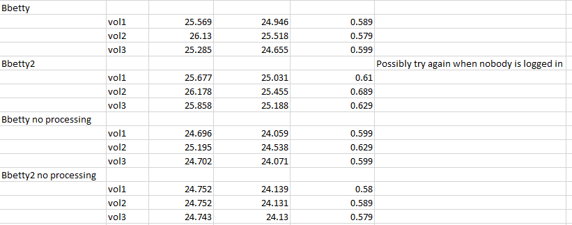
Welcome to my reflection for Lab 6. The task assigned for lab 6 was to test the performance of an algorithm meant to modify the volume of music samples. There were 3 versions of this algorithm that all had different approaches to this problem. This post will cover the results that my group and myself concluded to during our testing.
Test results:
Legend:
vol1 - First Algorithm
vol2 - Second Algorithm
vol3 - Third Algorithm
no processing - When the code that modified the music samples was commented out.


Before I discuss our results I will first cover how we conducted the tests. What we did was to run each version of the algorithm twice on all of the machines in the spreadsheet above. In addition we ran each algorithm with the volume modification code commented out. This was done so we can see how much of an impact that the volume modification code had on all of the machines tested. The algorithm times were obtained by using the command "time <application name>". What this did was run the application and at the end output how long it took to execute the program.
In terms of the results what stood out includes the following. First, was that on most of the machines each algorithm had similar times to each other, only deviating by around 1 or 2 seconds. The exception to this would be the Aarchie arm_64 machine as the second algorithm took at least 9 seconds in real time to complete when compared to the other algorithms that ran on that machine. Another finding that stood out, was that the ARM machines tested took around 27 to 62 seconds in real time to execute each of these algorithms but the xerxes x86_64 machine only took around 5 seconds in real time to complete each of these tasks. The last thing that stood out, was what happened when the volume modification code was commented out more specifically on the arm_64 machines. On most of the machines removing the volume mod code would shave off around 1 - 2 real time seconds in execution time. However, on the Aarchie machine removing that code cut execution time by around 4 - 13 real time seconds.
Monday, March 9, 2020
Lab 5 - Reflection
NOTE: The code written for the aarch_64 architecture was mostly done by my group members.
aarch_64 Code: https://gist.github.com/Megawats777/1344664ce18a295652ffbd1871482832
X86_64 Code: https://gist.github.com/Megawats777/0ace68a2dc077e8ca5d381cf3f3bcd81
Print character reference: https://stackoverflow.com/questions/8201613/printing-a-character-to-standard-output-in-assembly-x86
Welcome to my reflection on lab 5. This lab required us in several groups to get our feet wet with assembler programming for the aarch_64 and x86_64 architecture. The task we were given was to write a program that allowed the word "Loop" with a number to be printed 30 times. And we were required to write two versions of this program that worked with each of the architectures names previously. This blog entry will provide a overview between both versions of the program as well as my overall thoughts on programming in assembler for these newly encountered architectures.
The structure of the aarch_64 version of the program goes by the following. In the initialization stage there are two constants that determine the size of the loop. Continuing with initialization is where the "min" constant is loaded into the register x19 and the value 10 is loaded into the register x20. In the loop section, it starts off by taking the value in x19 and dividing it by 10 and storing both the remainder and the quotient into separate registers. The quotient is will act as the left digit and the remainder will act as the right digit. Once the digits are retrieved the number 48 is added on to them so that they can be displayed in ASCII format. Afterwards both digits are inserted into the correct slots in the "Loop:" message. However there is a check that ensures that if the left digit is a zero it won't be inserted. Once all the character processing is done the message with the numbers is printed. And at the end of the loop the value in x19 is incremented. To finish it off the program exits with a code 0.
The code for the x86_64 version of the program works similarly to the aarch_64 variant. However, the main difference is how the numbers are outputted. As compared to the aarch_64 version where numbers were inserted into the message, here the numbers are printed one by one. The way it works is that first I print "Loop:" then a space, then the first digit, the second digit, and finally a new line character. The actual printing of the individual characters works by first pushing the ASCII value or register containing the number I wanted to print onto the stack. Afterwards, I set the message location to be the memory location in the stack pointer. This will then tell the "sys_write" function what I want to print. And finally the desired character will be printed by calling "sys_write".
What stood out to me when coding for both architectures was how similar it was to writing code for the 6502 architecture. As in the 6502 I was managing registers and here I was doing the same thing just with more of them, in addition to more functionality being made available like division and modulus. In terms of debugging I would say it was a little bit easier as there were more community resources available to me like forum and blog posts. Now when comparing x86_64 and aarch_64, in terms of base coding structure they are quite similar except when it comes to the use of functions. As in aarch_64 for the most part you could use any register you wanted with any function but in x86_64 certain functions would only work if certain registers had specific values. The division function is a clear example of this, as in aarch_64 you could use any register you wanted as arguments. But for x86_64, you had to make sure that the rdx register was at zero and you could only divide the value in the register rax. Overall working on both architectures presented an interesting challenge and at the same time had demystified what its like to actually work on these chips at such a low level.
Subscribe to:
Posts (Atom)